Connecting Node-RED To PLCSIM Advanced

The first job in this project was simple to describe and awkward to achieve: make Node-RED talk reliably to Siemens PLCSIM Advanced. This article follows the real path into that work, from reading the Siemens API documentation and proving a console-only connection, through to the first bridge that made Node-RED a realistic option.

If you are new to Node-RED, the appeal of it is easy to understand once you have seen a few flows running. You can wire small pieces of logic together, inspect messages as they move, and build something useful without hiding everything inside one large program. For automation work, that is a very attractive way to experiment. You can start with a small idea, watch the data move, then improve the flow as your understanding improves.

PLCSIM Advanced has a similar pull from the PLC side. It lets you run a Siemens PLC virtually, test PLC logic without a physical CPU on the desk, and build training or development setups that would be expensive or awkward with real hardware. If you are learning Siemens automation, or trying to test a PLC project before commissioning, that is a useful capability.

So the natural thought is obvious enough: put Node-RED and PLCSIM Advanced together. Let Node-RED act as the visible, modular simulation layer around a virtual Siemens PLC. Use it to read PLC values, calculate simulated process behaviour, then write values back into the PLC. You get a PLC program running in PLCSIM Advanced, with Node-RED acting as a flexible soft simulation environment around it.

That was the direction of this project. The first article in the series is about the foundation needed before the interesting simulation work could begin.

Why This Problem Is Worth Solving

A basic PLC simulation usually begins with a very practical question: how do I make the PLC believe the plant exists?

That question sounds simple until you start building anything beyond a few forced bits. A PLC program usually expects signals to behave together. A pump status should follow the command in a believable way. A flow signal should rise when the pump runs and fall when the path is blocked. A tank level should climb or drop gradually. Pressure should respond to sources, restrictions, and changing demand.

You can force values manually for small tests, but manual forcing quickly becomes tiring. It also encourages very narrow testing. You prove that a permissive works, or that an alarm appears, but you do not get much confidence in how the wider control sequence behaves over time.

Flow through a process system is one of the first behaviours worth simulating because it connects so many parts of a PLC project together. A pump command, a motor running feedback, a valve position, a permissive, an interlock, a flowmeter, a totaliser, and a low-flow alarm can all be part of the same story. If the simulated flow never changes, or changes by hand only when someone remembers to force it, the PLC program is being tested in a very thin way.

A more useful simulation lets the process respond. If the virtual pump starts, the flow should rise. If a valve closes, the flow should fall or stop. If two sources feed the same line, the resulting value should follow the rule the model has been given. That kind of behaviour gives you a better test of sequences, alarm delays, restart logic, operator displays, and edge cases that are awkward to create with a real plant.

There is also a practical commissioning reason for doing this. Many PLC faults are discovered late because the real mechanical process is the first time the control code sees believable signal behaviour. A soft flow simulation will never replace real commissioning, but it can move a lot of basic logic testing earlier. You can find spelling mistakes, missing interlocks, inverted assumptions, awkward alarm behaviour, and weak restart handling while the PLC is still running virtually.

For training, the benefit is different but just as useful. A beginner can see how a PLC program reacts when the process changes. They can watch a value ramp, see a valve restrict it, and connect that behaviour back to the PLC logic. That is far more useful than staring at a static tag table full of forced values.

That is where Node-RED becomes interesting. It gives you a place to build soft plant behaviour in small, visible pieces. You can keep the PLC program in the Siemens world where it belongs, while Node-RED handles the surrounding process signals. A simulation can start small with one read and one write, then grow into flowmeters, tanks, pressures, and analog instruments.

For someone learning, the value is even stronger. Node-RED makes the data path visible. You can see the incoming PLC values, the calculated result, the staged output, and the final write back to the virtual PLC. That visibility helps you build the mental model of what the PLC is doing and what the simulated plant is doing around it.

The challenge was that Node-RED and PLCSIM Advanced do not naturally meet in the middle. Node-RED runs on Node.js and is usually extended with JavaScript packages. PLCSIM Advanced exposes a Siemens API intended for the Windows and .NET side of the world. The project needed a clean crossing point between those two environments.

What Node-RED And PLCSIM Advanced Each Bring

It helps to separate the two tools before looking at the integration.

Node-RED is very good at orchestration. A flow can receive a message, shape it, pass it through a calculation, store values in context, and send the result somewhere else. It is also very approachable. You can open the editor, drop in a few nodes, wire them together, and inspect what is happening without building a full application from scratch.

That makes Node-RED a good fit for simulation logic. A simulation flow often has clear stages:

• poll live PLC values
• look up cached tag values
• calculate a simulated process value
• stage outputs for writing
• flush the output values back to the PLC

PLCSIM Advanced brings the virtual PLC. It can run a Siemens PLC instance on the engineering machine and expose that instance through Siemens’ runtime interface. The useful operations include finding PLC instances, connecting to a selected instance, loading symbolic tags, reading values, and writing values back.

Those two strengths fit together well at the system level. The PLC can keep running the control program. Node-RED can supply the surrounding process behaviour. The awkward part sits at the API level. The Siemens PLCSIM Advanced API belongs to a different runtime world from a normal JavaScript library.

A useful way to picture the design we were heading toward is this:

That shape became the foundation of the package. The early work was about proving each part of that route before building higher-level simulation nodes on top of it.

Research The Siemens Side

The first serious question was about the Siemens side of the problem. PLCSIM Advanced was running a virtual PLC, but a running virtual PLC is only useful to an external tool if there is a supported way to talk to it. The Siemens help files became the starting point.

The documentation pointed toward the runtime manager, the endpoint used to connect to it, and the API assembly installed with PLCSIM Advanced. In the working console project, that assembly was referenced as `Siemens.Simatic.Simulation.Runtime.Api.x64.dll` from the Siemens PLCSIM Advanced API folder. The examples in the help material were written for languages such as C#, which made sense for the Siemens API. The Node-RED route still had to be designed.

That was the first real boundary. Node-RED is a JavaScript and Node.js environment. The Siemens route into PLCSIM Advanced was a Windows API route with C# examples and a Siemens DLL. At that stage, the task was less about Node-RED nodes and more about answering a basic engineering question: can we build any local tool that talks to PLCSIM Advanced reliably?

I used ChatGPT, and later Codex, as part of that research, with the Siemens documents available as context, to sanity-check whether there was a reasonable way for Node-RED to connect directly. The useful suggestion was to stop trying to make Node-RED speak to the Siemens DLL itself and build a small local bridge instead. That turned into a very direct request: help me build a simple console application that can connect to the runtime manager, list instances, attach to the right virtual PLC, read values, and write values. If that worked, the console application could become our own local API between Node-RED and PLCSIM Advanced.

That changed the shape of the work. The first target was no longer a Node-RED node. The first target was a console-only proof that the Siemens API could be reached and controlled from a small local program.

Build The Console Connection Test

The console project that came out of this stage was the real bridge before the Node-RED package existed. It began as a deliberately small Codex-assisted build, not as a big application plan. The aim was simple: create a console tool that proves the connection path cleanly. It targeted .NET Framework 4.8, referenced the Siemens runtime API DLL, and focused on the first operational question: if someone gives this tool a PLCSIM Advanced endpoint, can it get to the right virtual PLC without guesswork?

That connection point matters more than it may sound at first. The console app was not connecting straight to a tag or straight to one named PLC. It first had to connect to the runtime manager. You can think of the runtime manager as the place that knows which simulated PLC instances currently exist on that machine. Until the tool could reach that manager and ask for its registered instances, every later tag idea was still hypothetical.

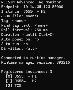
So the workflow became very practical. Ask Codex for the smallest useful console proof, then make that proof do one honest job at a time: start with an endpoint, try the connection, ask what instances are registered, and choose the one you actually want. In the tag monitor project, that shape shows up clearly in both the command-line options and the interactive wizard. The tool prompts for an endpoint, tries to connect, shows the runtime manager version, prints the available instances, then lets you select the one you want to work with.

That sequence was useful because it matched the way people actually troubleshoot these setups. If the endpoint is wrong, you want to know immediately. If the runtime manager answers but no instances are registered, that is a very different problem. If the correct PLC exists but you pick the wrong one, the connection has technically succeeded but the test is still aimed at the wrong target. The console app made those states visible in a very plain way.

A simple example helps here. Imagine opening the tool and entering the endpoint for the runtime manager. The first good sign is that the runtime manager answers at all. The second is that it reports a sensible version and shows a list of registered virtual PLCs. The third is that you can pick the correct instance from that list and attach to it cleanly. At that point, you have something much more valuable than a vague feeling that the API might work. You have a repeatable path into the correct virtual PLC.

The earliest useful console output was deliberately plain. It showed the endpoint being used, whether the runtime manager connection succeeded, the runtime manager version, the available instances, and the selected instance. Those details are not glamorous, but they are the exact details you need when a simulation setup refuses to behave. A clean list of what the tool found is far more helpful than a black box that simply says the connection failed.

This also began to shape the tone of the whole project. The bridge was never meant to be clever for its own sake. It was meant to make the Siemens side understandable. A good console connection test tells you where you are connected, what PLCSIM Advanced instances exist, and which one you are about to use. That clarity is part of the value.

At this point, the system was still a console application rather than a Node-RED flow. That was the right order. The Siemens connection path needed to be proven cleanly before Node-RED was added on top of it. Once the console app could do this reliably, Node-RED stopped feeling like a risky jump and started feeling like the next sensible layer.

This is an important pattern in automation tooling. When a future integration has several moving parts, prove the awkward vendor-facing layer by itself first. Then bring the nicer orchestration layer in once the difficult boundary is understood.

Read And Write A Real Tag

Connecting to the runtime manager proved the Siemens doorway was real. The next question was more demanding: once attached to a virtual PLC, could the console app actually find a real symbolic tag, understand what kind of value it was dealing with, and read something meaningful back?

That became the next Codex-assisted build step. The request was no longer just “can we connect?” It was “can we make this connection useful?” In practice that meant teaching the console tool how to refresh the symbolic tag list from the selected instance, search that list for something recognisable, choose a target tag, and start reporting its live value in a way a human could trust.

That tag list refresh mattered because a connected PLC is still a black box until you can see its symbolic surface. Once the monitor could refresh the available tags, you were no longer guessing at whether a tag path existed or whether you had spelled something correctly. You could search by a piece of a name, narrow the result, and work from what the PLC actually exposed rather than what you hoped it exposed.

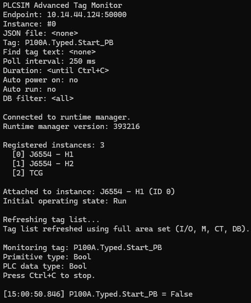
The first useful read workflow was deliberately grounded. Attach to the chosen PLCSIM Advanced instance. Refresh the tag list. Pick a known symbolic tag. Report its primitive type and PLC data type. Then sit and monitor the value at a steady interval. That may sound modest, but it was the first moment the bridge felt alive. The tool was no longer merely reaching Siemens software. It was observing a real part of the simulated control system from outside the Siemens editor.

A simple example helps here too. If the selected tag is a boolean pushbutton or run signal, the value stream should make sense immediately. You are looking for something human-readable and believable: true or false, changing when you expect it to change, staying steady when the system is quiet, and matching what the virtual PLC is actually doing. If that basic observation cannot be trusted, there is no point building anything more ambitious on top of it.

Once reading worked, writing became the next checkpoint. A tool that can only observe the PLC is useful for diagnostics, but it cannot yet simulate plant behaviour. To make a virtual PLC behave as if a plant exists around it, the outside tool has to write believable values back into the simulation. That is where the bridge stops being a viewer and starts becoming an active participant.

The early write tests stayed intentionally small. Pick a sensible tag. Write a value. Read it back. Confirm that the name resolution, data type handling, and returned value all line up with expectation. This was not about showing off a large feature. It was about proving that the whole route held together when something real moved in both directions.

That step also answered an important design question for the later Node-RED work. If a small console app can reliably refresh tags, locate one symbolic point, read it, and write it back, then Node-RED does not need to carry the Siemens complexity itself. Node-RED can stay focused on orchestration. The bridge can own the awkward vendor-facing work and return a result in a shape the flow can actually use.

In hindsight, this was the moment the bridge stopped feeling theoretical. Phase 2 proved that the correct PLC could be found. Phase 3 proved that the PLC could be interacted with in a meaningful way. That is a much more interesting milestone, because it is the first point where a process simulation starts to feel possible rather than merely imaginable.

Tie Tags Together Into A Scenario

Before I even started the Node-RED side, I wanted to know whether the Siemens API was capable of successive reads and writes while the connection stayed open. There was very little appeal in opening and closing a PLC connection for every small action. That would become heavy quickly, especially once a simulation needed to keep checking values and feeding updated ones back. The bridge needed to feel more like an active session than a disposable one-shot command.

Single tag reads and writes were enough to prove the API path, but they were not enough for the question I actually cared about. Could the connection stay open and keep working, cycle after cycle, without needing to reconnect every time? That is much closer to the real job. A process simulation is a steady rhythm of reads, small decisions, and writes over time. For one flow instrument that might mean watching a pump running bit, checking that the instrument is in simulation mode, and then writing the value the PLC should see. A level model would need its own set of related signals.

That was the point where the console app moved beyond tag monitoring. I asked Codex to help scaffold a small JSON configuration system so I could define the PLC tags involved and the rule that connected them. The first relationship I had in mind was intentionally plain. If the pump was running, the flow indication should sit at 20.0. If the pump stopped, the flow should fall back to 0.0. That was enough to prove whether the bridge could stay connected and keep the relationship running.

JSON was a deliberate choice. Node-RED already handles JSON comfortably, so it made sense to shape the bridge inputs that way from the start. If the bridge could parse that configuration now, some of the same structure might carry forward into the Node-RED side later. Even if the final format changed, the thinking would still be useful.

A stripped-back configuration for that first proof looked something like this:

{
  "description": "Simple pump to flow proof",
  "connection": {
    "instance": "J6554 - H1"
  },
  "signals": {
    "pumpRunningTag": "P100A.Typed.Running",
    "simulationEnableTag": "IF100.Typed.Simulate",
    "flowOutputTag": "IF100.Typed.Generic_Analog_Data.Soft_Sim_Value"
  },
  "behaviour": {
    "runningFlow": 20.0,
    "stoppedFlow": 0.0
  }
}

What I liked about that shape was that it stayed readable. One part named the PLC points. Another part described what should happen between them. Once that was written down, I was no longer poking random tags to see what happened. I was describing a small piece of plant behaviour in a form the bridge could repeat.

That put the work on much firmer ground. Real process testing is about relationships. Does the pump state affect the flow the way you expect? Does the instrument move when it should? Do the permissives and alarms around it behave properly? A small JSON file was enough to start asking those questions in a consistent way, while the bridge kept the connection alive in the background.

Use The Console App As A Bridge

This is where the Node-RED idea became practical again. The console app had already shown that the Siemens-facing side could be handled locally. The next check was the round trip between Node-RED, the bridge, and PLCSIM Advanced, with the result coming back in a shape the flow could actually use.

That bridge shape gave each side a sensible role:

• Node-RED would own the flow, the visual orchestration, and later the user-facing nodes.
• The console bridge would own the Siemens API calls and the PLCSIM Advanced connection details.
• The request and response shape would become the contract between them.

The first Node-RED-facing shape could be simple. Node-RED could call the console bridge, pass in a structured request, and read the result. That is why the console work was so valuable. It gave Node-RED a local API of our own for PLCSIM Advanced work.

There was still more work to do after that. A one-shot console call is useful for connection checks and proofs, but cyclic simulation wants something that can stay alive, keep state, and respond repeatedly. That is where the later maintained session host and `plcsim-session` node came from. The session layer grew out of the console bridge proof.

By the end of this foundation stage, Node-RED had a believable route into PLCSIM Advanced. The route had been proven from the Siemens side first, then shaped into something Node-RED could call with confidence.

What This Foundation Meant

The first five foundation stages are infrastructure work, but they are also the part of the story that explains why the later Node-RED package could exist at all.

At this stage, the project had five useful proofs:

• The Siemens runtime manager endpoint could be reached from a local tool.
• The available PLCSIM Advanced instances could be listed and selected.
• The selected virtual PLC could be attached to through the Siemens API.
• Real symbolic tags could be refreshed, searched, read, and written.
• Related tags could be grouped into process scenarios that started to resemble useful simulation behaviour.

That foundation is what lets the package move into safer Node-RED reads and writes later in the build. It also explains why the early work was deliberately methodical. A useful simulation system needs reliable connection handling and tag awareness before it needs clever process models.

For someone beginning with Node-RED and PLCSIM Advanced, this is the order that made the work feel manageable:

1. Reach the runtime manager. If the Siemens runtime manager cannot be reached reliably, nothing further is trustworthy yet.
2. Resolve the right PLC instance. More than one virtual PLC can exist on an engineering machine, so the target needs to be selected deliberately.
3. Load the tag surface. Work from the symbolic tags the PLC actually exposes instead of guessing names from memory.
4. Read one value cleanly. A single believable read proves you can observe the virtual PLC in a meaningful way.
5. Write one value back. A single believable write proves you can influence the simulated plant side as well as inspect it.
6. Group related tags into behaviour. Once the basics are solid, relationships like pump-to-flow or inflow-to-level become much easier to build and debug.

The later sections of this build move on from that base. They move from connection and tag knowledge into single reads, batch polling, buffered writes, flowmeter simulation, level modelling, generic analog behaviour, pressure curves, structured editor design, and long-run performance lessons.

The beginning is quieter than the later simulation work, but it is the part that makes the later work dependable.

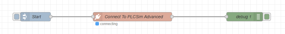
The First Node-RED Proof Was A Simple Connection Check

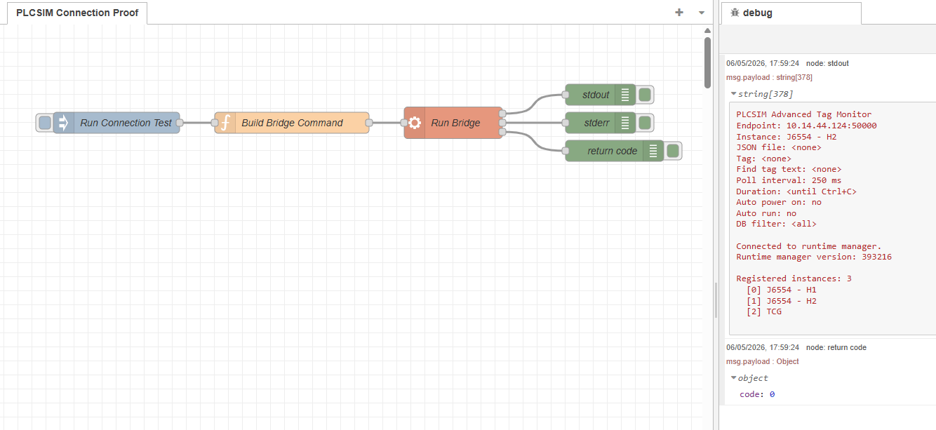
The first Node-RED proof was much simpler than the later setup. I asked Codex to help write a small function-driven bridge call that pointed at the helper executable by absolute path, asked it to check J6554 - H2, and pushed the result back into the flow.

In other words, the first question inside Node-RED was the same question the console app had already answered outside it: can I reach the runtime manager, can I see the PLC instance I care about, and can I get that answer back in a clear result?

const bridgeExe = 'C:\\Tools\\PLCSIM Advanced Tag Monitor\\PLCSIM Advanced Tag Monitor.exe';
const endpoint = '10.14.44.124:50000';
const instanceName = 'J6554 - H2';

msg.payload = '"' + bridgeExe + '" --endpoint ' + endpoint + ' --instance "' + instanceName + '" --list';
return msg;

The function node assembled the bridge call, an exec step could run it, and the returned output came back on msg. That was enough to prove the handshaking between Node-RED and the bridge application.

Once that connection test worked, the next request was the tag list, and that is the point where a connection check starts becoming useful, because a successful handshake tells you the door is open, while the symbolic tag list tells you what is actually available on the other side of it.

At this point there was no shared cache yet, only the msg object carrying the result of the connection test. The tag-list step came next because once Node-RED could ask for that list and receive it back cleanly, it became possible to think more seriously about how that information should be kept inside the flow.

The real attraction of storing the tag list was not convenience for its own sake. It was that reads and writes would soon need a proper reference point. If a requested tag name was wrong, it would help to know that immediately. If a tag was present in the list but had not been read yet, that was a different issue. Those distinctions only became possible once the tag list was kept somewhere stable.

The next realisation followed quite quickly. A Node-RED flow could trigger the bridge, get a result back, and move on, but it could not hold a PLC session open in the way this work really needed. Even with looping messages, there was no clean way to treat that connection as a live thing inside the flow itself.

The next stages were never going to be one request every now and then. They were going to be repeated reads, repeated writes, and eventually faster cyclic behaviour. If every step meant opening the door again, doing one small job, and closing it again, that would become awkward very quickly.

This is where the limit of Node-RED became clear. The flow could prove that the bridge worked, but it could not be the place where a long-lived PLC session lived. That meant finding a different way to keep the session active.

Read A Tag, Change It, Write It Back

Single reads and writes were the next thing I tested, but I started in the simplest possible way: read one tag, change that value in the flow, then write it straight back to the PLC as an immediate write.

At this point the configuration node still was not in place, so the flow itself carried the whole sequence:

connect -> read -> modify -> write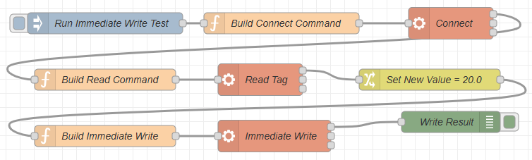

That was the chain I wanted to prove inside Node-RED before going any further. It was not enough to know that the bridge could connect, and it was not enough to know that a tag list could be returned. I wanted to see the full read and write path work end to end inside one flow.

First connect to the right PLC instance. Then ask for a real tag value. Then modify that value in Node-RED. Then send the changed value back through the bridge to the PLC. If that whole path held together, it meant Node-RED could participate in the PLC conversation properly instead of only checking whether the door was open.

This all worked fine. Node-RED could establish the full chain of events for reading and writing, and that gave the project the confidence to keep moving.

Keeping The PLC Instance Alive

Once the first read and immediate write worked, the next question was whether the same idea could run circularly. I needed to be able to start the system up, keep the connection active, and then perform reads and writes from a defined configuration instead of rebuilding the whole interaction for every single step. I tried plenty of different flow variations to make that happen, but the only part that stayed reliable was the initial read and write proof. After that, I kept running into issues.

That is where the first function-node proof started to run out of road. A flow could trigger the bridge, get a result back, and move on, but it was not a good place to keep a PLC instance present as a live session. The more this leaned toward repeated polling and repeated writes, the more obvious that became.

I asked Codex to help me create what I was thinking of as a context node, meaning something that could hold onto that shared PLC state between different nodes. Once the idea was turned into real Node-RED nodes, that role settled into what became the system node. The answer that came back was that this was probably the point where a proper contrib package became the more feasible route.

From that point on, the work started to look less like one stretched-out experiment and more like the start of a proper toolset. The first piece was a system node to hold the shared PLC state. Alongside that came a basic connect node. Those parts gave the connection somewhere stable to live and gave the rest of the flow something solid to build on.

{
  "_msgid": "0e80c4e10b391a18",
  "payload": {
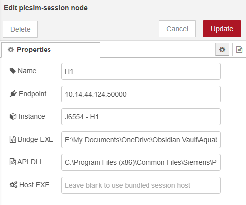
    "active": true,
    "runtimeConnected": true,
    "endpoint": "10.14.44.124:50000",
    "instanceName": "J6554 - H1",
    "instanceFound": true,
    "matchedInstance": "J6554 - H1",
    "runtimeManagerVersion": "393216",
    "instanceCount": 3,
    "instances": [
      "J6554 - H1",
      "J6554 - H2",
      "TCG"
    ],
    "rawError": "",
    "exitCode": 0,
    "status": "Connected to 10.14.44.124:50000 for J6554 - H1."
  },
  "topic": "",
  "runtime": {
    "active": true,
    "runtimeConnected": true,
    "endpoint": "10.14.44.124:50000",
    "instanceName": "J6554 - H1",
    "instanceFound": true,
    "matchedInstance": "J6554 - H1",
    "runtimeManagerVersion": "393216",
    "instanceCount": 3,
    "instances": [
      "J6554 - H1",
      "J6554 - H2",
      "TCG"
    ],
    "rawError": "",
    "exitCode": 0,
    "status": "Connected to 10.14.44.124:50000 for J6554 - H1."
  }
}

The returned payload showed the next big improvement very clearly. The connection was active, the runtime manager was reachable, the requested PLC instance had been found, and Node-RED now had a structured result it could work with directly.

system node -> connect -> read / write

The system node was the key part of that shift in approach. If Node-RED was going to do this circularly, it needed somewhere stable for that PLC relationship to live. Once that existed, the rest of the nodes could stop acting like isolated tests and start acting like parts of one running system.

Browse The PLC Once, Then Work From Known Tags

Once the system node and connection node were in place, the next question was straightforward: now that we could connect, could we poll the PLC for all of the available tags?

That step was important for a very practical reason. I did not want Node-RED attempting reads and writes blindly. If a tag string was malformed, pointed at the wrong place, or simply did not exist in the selected PLC instance, I wanted to know that before a read or write step even tried to run.

The logic I had in mind was fairly simple. Connect once. Browse the available tags once. Hold those tag strings in memory. Then compare the tags listed in a file or configuration against that known list before trying to use them. That way, the flow could warn me early that a tag name was wrong instead of failing later in a less obvious place.

connect -> browse tags -> hold tag list in memory -> validate requested tags -> read / write

That was the point where we needed a dedicated Browse Tags node. I asked Codex to develop it and add it to the contrib package so the tag-list step could become a proper reusable part of the toolkit rather than another one-off experiment.

I could have written all of that myself with enough time, but using Codex was a quick and genuinely useful way to get these first building blocks together. For this stage of the project, that was exactly what I needed. Here is the actual output for the tag browse block in the contrib package, the plcsim-tags-cache node:

"use strict";

const bridge = require("../lib/plcsim-bridge");
const status = require("../lib/plcsim-status");

module.exports = function (RED) {
    function PlcSimTagsCacheNode(config) {
        RED.nodes.createNode(this, config);
        const node = this;
        const session = RED.nodes.getNode(config.session);

        node.session = session;
        node.endpoint = config.endpoint || bridge.DEFAULT_ENDPOINT;
        node.instanceName = config.instanceName || bridge.DEFAULT_INSTANCE_NAME;
        node.contextKey = config.contextKey || bridge.DEFAULT_CONTEXT_KEY;
        node.dbFilter = config.dbFilter || "";
        node.apiAssemblyPath = config.apiAssemblyPath || bridge.DEFAULT_API_ASSEMBLY_PATH;
        status.update(node, {});

        node.on("input", async function (msg, send, done) {
            send = send || function () {
                node.send.apply(node, arguments);
            };

            if (session) {
                const contextKey = bridge.firstNonEmptyString(
                    msg.contextKey,
                    node.contextKey,
                    bridge.DEFAULT_CONTEXT_KEY
                );
                const dbFilter = bridge.normaliseDbFilter(
                    bridge.firstDefined(msg.dbFilter, node.dbFilter, "")
                );

                status.update(node, { fill: "blue", shape: "dot", text: "loading tags" });

                try {
                    const result = await session.loadTags(dbFilter);
                    const summary = bridge.buildTagsSummary(result, {
                        endpoint: session.endpoint,
                        instanceName: session.instanceName,
                        contextKey: contextKey
                    });

                    if (summary.runtimeConnected && summary.instanceFound && result.tagsGzipBase64) {
                        const tags = bridge.decodeTagsPayload(result.tagsGzipBase64);
                        const globalContext = node.context().global;

                        globalContext.set(contextKey, tags);
                        globalContext.set(contextKey + ".meta", {
                            endpoint: summary.endpoint,
                            instanceName: summary.instanceName,
                            tagCount: tags.length,
                            loadedAt: result.loadedAt || null,
                            dbFilter,
                            sampleTags: Array.isArray(result.sampleTags) ? result.sampleTags : []
                        });

                        summary.active = true;
                        summary.stored = true;
                        summary.tagCount = tags.length;
                        summary.status = "Stored " + tags.length + " tags in global context key '" + contextKey + "'.";
                    } else {
                        summary.status = "Failed to load tags for " + (summary.instanceName || summary.endpoint) + ". " + (summary.rawError || "No additional error text.");
                    }

                    msg.payload = summary;

                    status.update(node, {
                        fill: summary.stored ? "green" : summary.runtimeConnected ? "yellow" : "red",
                        shape: "dot",
                        text: summary.stored ? summary.tagCount + " tags cached" : "tag load failed"
                    });

                    send(msg);
                    done();
                } catch (error) {
                    status.update(node, { fill: "red", shape: "ring", text: "error" });
                    done(error);
                }

                return;
            }

            const endpoint = bridge.firstNonEmptyString(
                msg.endpoint,
                typeof msg.payload === "string" ? msg.payload : "",
                node.endpoint,
                bridge.DEFAULT_ENDPOINT
            );
            const instanceName = bridge.firstNonEmptyString(
                msg.instanceName,
                msg.plcName,
                msg.plc,
                node.instanceName
            );
            const contextKey = bridge.firstNonEmptyString(
                msg.contextKey,
                node.contextKey,
                bridge.DEFAULT_CONTEXT_KEY
            );
            const apiAssemblyPath = bridge.firstNonEmptyString(
                msg.apiAssemblyPath,
                node.apiAssemblyPath,
                bridge.DEFAULT_API_ASSEMBLY_PATH
            );
            const dbFilter = bridge.normaliseDbFilter(
                bridge.firstDefined(msg.dbFilter, node.dbFilter, "")
            );

            const request = {
                endpoint,
                instanceName,
                contextKey,
                apiAssemblyPath,
                dbFilter
            };

            status.update(node, { fill: "blue", shape: "dot", text: "loading tags" });

            try {
                const result = await bridge.runBridgeScript("Get-PlcSimTags.ps1", request);
                const summary = bridge.buildTagsSummary(result, request);

                if (summary.runtimeConnected && summary.instanceFound && result.tagsGzipBase64) {
                    const tags = bridge.decodeTagsPayload(result.tagsGzipBase64);
                    const globalContext = node.context().global;

                    globalContext.set(contextKey, tags);
                    globalContext.set(contextKey + ".meta", {
                        endpoint,
                        instanceName,
                        tagCount: tags.length,
                        loadedAt: result.loadedAt || null,
                        dbFilter,
                        sampleTags: Array.isArray(result.sampleTags) ? result.sampleTags : []
                    });

                    summary.active = true;
                    summary.stored = true;
                    summary.tagCount = tags.length;
                    summary.status = "Stored " + tags.length + " tags in global context key '" + contextKey + "'.";
                } else {
                    summary.status = "Failed to load tags for " + (instanceName || endpoint) + ". " + (summary.rawError || "No additional error text.");
                }

                msg.payload = summary;

                status.update(node, {
                    fill: summary.stored ? "green" : summary.runtimeConnected ? "yellow" : "red",
                    shape: "dot",
                    text: summary.stored ? summary.tagCount + " tags cached" : "tag load failed"
                });

                send(msg);
                done();
            } catch (error) {
                status.update(node, { fill: "red", shape: "ring", text: "error" });
                done(error);
            }
        });
    }

    RED.nodes.registerType("plcsim-tags-cache", PlcSimTagsCacheNode);
};

What really stood out here was that this worked first time. Codex had also taken the extra step of writing the returned tags into Node-RED global context, which was not something I had properly thought through at that point.

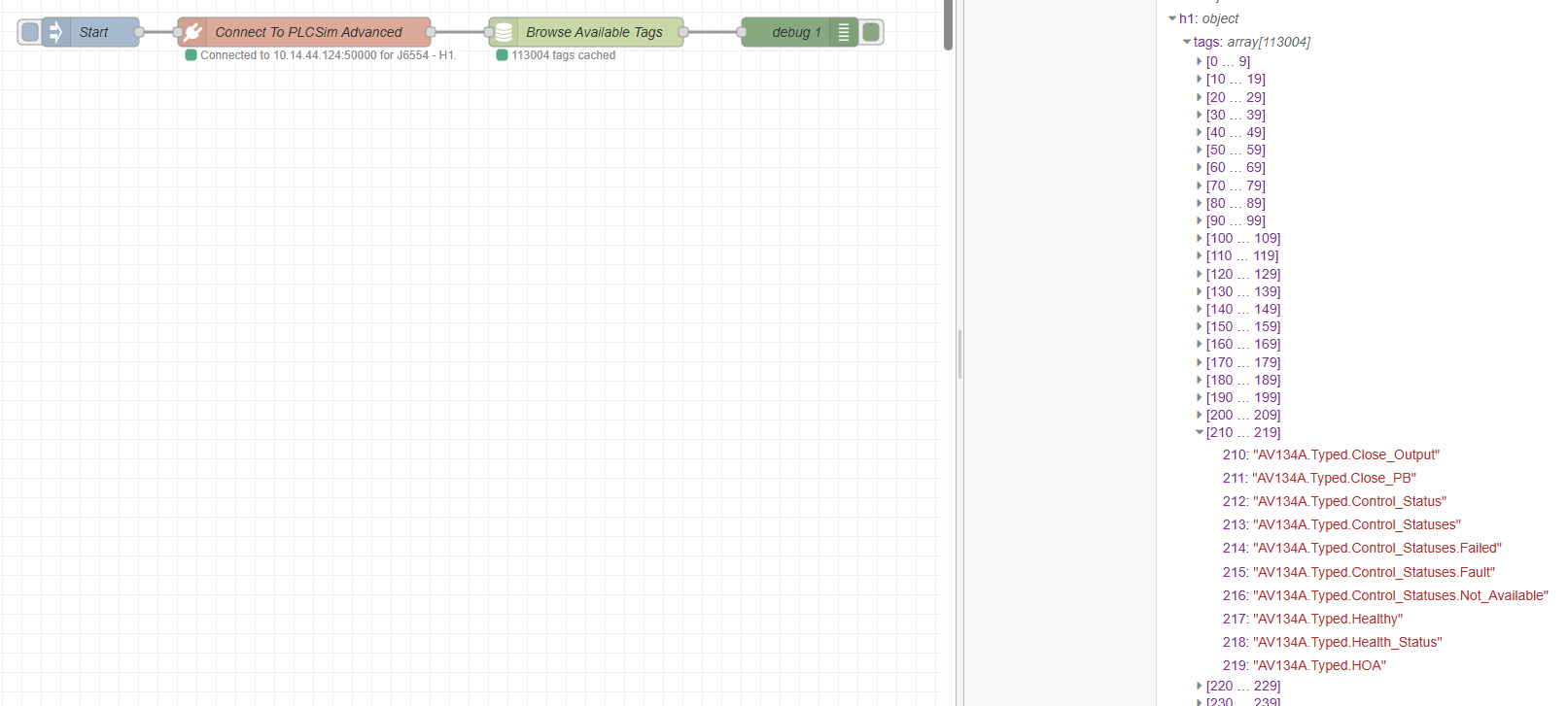
That was extremely useful. It meant the browse step was not only returning a result for that one moment, it was also leaving behind something the rest of the system could keep using. It gave me an early warning if a tag name was malformed or missing, and it did that before a later read or write step had the chance to fail in a less obvious way.

Once that node existed, the package could start building a known picture of what the PLC actually exposed. A read node could check whether a requested tag existed before trying to fetch it. A write node could do the same before sending a value back. Even before any simulation logic became more advanced, that made the whole setup feel far more dependable.

The First Cyclic Read Flow

Once the connection and tag browsing were in place, the next thing I wanted was the first real cyclic simulation flow. I asked Codex for a function-node-driven flow that would read a flowmeter, check the running state and speed of the related pumps, form a simple linear relationship, write the simulated flow value back, wait a short period, and then do it again.

The first example I used was IF201. The idea was simple enough to explain. If P201A or P201B was running above zero percent, then the flowmeter should rise between its minimum and maximum scale in line with the pump speed. If the pump speed increased, the simulated flowmeter value should increase with it.

To do that, the flow had to read several live values from the PLC before it could calculate anything sensible. It needed the flowmeter scale from tags such as IF201.Typed.Generic_Analog_Data.Scale_Max and IF201.Typed.Generic_Analog_Data.Scale_Min. It also needed the pump range from tags such as P201A.Typed.Max_Speed and P201A.Typed.Min_Speed. From there, it could build the relationship between P201A.Typed.Actual_Speed and IF201.Typed.Generic_Analog_Data.Soft_Sim_Value.

That was a small but important change in complexity. Up to this point, a lot of the proof work had been about one request and one response. This flow needed multiple reads from the simulated PLC, one calculation step in the middle, and then a write back at the end.

At that stage the dedicated plcsim-read and plcsim-write nodes did not exist yet, so I asked Codex to develop the whole thing as a flow. The connection step was already handled by the contrib connection node, and the tag browsing step was already handled by the contrib browse-tags node. What came next was the first repeatable cycle built on top of them.

connect -> browse tags -> read required tags -> calculate linear relationship -> write flowmeter value -> delay -> repeat

The read step needed its own configuration JSON so a function node could know which tags to request and how to group them. Once those values were returned, the function could compare the live pump speed against the configured minimum and maximum, scale that into the flowmeter range, and then send the new simulated value back to the PLC.

//Pull config for IF201
let c = {}
c = {
      "id": "if201-flow-from-p201a-or-p201b",
      "type": "analog-scale",
      "enabled": true,
      "sourceSelector": "highest",
      "sources": [
        {
          "name": "P201A",
          "kind": "vsdPercent",
          "valueTag": "P201A.Typed.Actual_Speed",
          "weight": 1.0
        },
        {
          "name": "P201B",
          "kind": "vsdPercent",
          "valueTag": "P201B.Typed.Actual_Speed",
          "weight": 1.0
        }
      ],
      "output": {
        "valueTag": "IF201.Typed.Generic_Analog_Data.Soft_Sim_Value",
        "scaleMinTag": "IF201.Typed.Generic_Analog_Data.Scale_Min",
        "scaleMaxTag": "IF201.Typed.Generic_Analog_Data.Scale_Max",
        "softSimSelectTag": "H2_Soft_Sim_Select.IF201"
      },
      "options": {
        "clampInput": true,
        "clampOutput": true,
        "fallbackToScaleMinWhenNoPumpActive": true,
        "smoothingSeconds": 10.0,
        "rangeCap": 90
      }
}

msg.config = c
return msg;

This little block carried a lot of the thinking for that first cyclic flow. The sources section named the two pumps that could drive the instrument, and each one pointed at its live speed tag. The sourceSelector was set to highest, which meant the logic would work from whichever pump was currently making the stronger contribution.

The output section pointed at the flowmeter tags that defined the final result. Soft_Sim_Value was the tag to be written back. Scale_Min and Scale_Max told the flow what engineering range the instrument should use. The soft-simulation select tag was there so the PLC side could know this instrument was being driven by the simulation path.

The options section provided additional controls around how that relationship behaved. Input and output clamping stopped the calculation wandering past sensible bounds. Falling back to the scale minimum when no pump was active kept the instrument from drifting when it should be quiet. The smoothing value stopped the result stepping too abruptly, and rangeCap gave the relationship a ceiling before it reached the full scale.

What I liked about this was that the flow logic no longer had to guess what relationship it was supposed to build each time. The JSON named the sources, named the destination, and described the limits of the calculation in one place. That made the cyclic read and write loop much easier to reason about.

1. Read the tags required for the relationship.
2. Perform the linear relationship check.
3. Write the calculated value to the flowmeter simulation tag.
4. Wait for a short period.
5. Repeat the cycle.

This was really the birth point of the later plcsim-read and plcsim-write nodes. Before they were packaged as dedicated nodes, they existed as a practical need inside this first cyclic flow. The flow had to read a known set of values, perform one clear piece of process logic, and then write the result back in a form the PLC could consume.

Moving To Batch Management

The first cyclic flow proved the simulation idea, but it also exposed the next problem very quickly. One read and one write could work. Several reads and writes landing together were a different story. The supporting bridge would start to fall over when multiple requests arrived at the same time, and that was exactly where the design was heading.

My Node-RED design was meant to be modular. I wanted separate loops for separate asset relationships, because that fitted the application I was building. One loop could look after a flowmeter relationship. Another could look after a level. Another could handle pressure. That was a good shape inside Node-RED, but it also meant those loops would often wake up together, and when they did they would all try to talk to the bridge together as well.

So the single-read and single-write approach had to give way to batch management. The PLC side needed one place to control overlap, one place to gather live values, and one place to send writes back in a clean order.

connect -> browse tags -> batch read -> global live buffer -> simulation loops -> write queue -> batch write

I already had all of the tag names cached, which meant the next step was to separate PLC traffic from simulation logic. The dedicated read loop could poll the tags that were actually needed and store the latest values in a buffer held in Node-RED global context. The simulation loops could then read from that buffer instead of hitting the PLC directly. After each pass, they could queue any output changes into a basic write array for the dedicated write loop to flush back through the bridge.

This split made the responsibilities much clearer. The batch read loop gathered the current PLC state. The simulation loops used that buffered state to calculate relationships such as pump speed to flow. The batch write loop handled the write-back path so those simulation loops were no longer competing with each other or piling requests on top of the bridge at the same moment.

That was the point where I asked Codex to create dedicated plcsim read batch and plcsim write batch nodes. Those nodes became the control point that let the Node-RED side stay modular while the PLC side stayed orderly.

1. Connect once and browse the available tags.
2. Start a dedicated batch-read cycle for the tags the simulation actually needs.
3. Store the latest values in a global buffer that any simulation loop can use.
4. Let each simulation loop calculate independently and queue its output writes.
5. Use one batch-write path to send those queued values back cleanly.

Once that structure was in place, the design had room to grow. The PLC traffic became predictable, the simulation loops stayed independent, and the whole thing was much better suited to continuous operation instead of one-off proof steps.

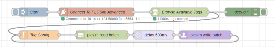
Tag Config And The First Batch Read

Once the batch approach was clear, the next question was what the read loop should ask for on each acquisition pass. The Tag Config function built that list, then passed it forward on msg.tags so the batch-read node could poll that defined set of PLC values on every cycle.

{
  "tags": [
    "P201A.Typed.Running_In_Auto",
    "P201A.Typed.Actual_Speed",
    "P201A.Typed.Running",
    "P201B.Typed.Running_In_Auto",
    "P201B.Typed.Actual_Speed",
    "P201B.Typed.Running",
    "IF201.Typed.Scaled_Value",
    "IF201.Typed.Generic_Analog_Data.Soft_Sim_Value",
    "IF201.Typed.Generic_Analog_Data.Scale_Min",
    "IF201.Typed.Generic_Analog_Data.Scale_Max",
    "H2_Soft_Sim_Select.IF201",
    "AV205.Typed.Open_IND"
  ]
}

The pump tags gave the running state, auto state, and actual speed for both drives. The flowmeter tags gave the current scaled value, the soft simulation value being written by Node-RED, and the engineering range defined by the minimum and maximum scale. The soft-simulation selector showed whether the instrument was switched into the path where that simulation value could take over. The valve indication sat alongside those tags so the wider process state could also be checked as the flow developed.

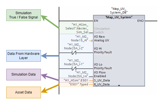
The soft-simulation selector deserves a quick explanation here. Soft simulation is a mode that allows the scaled instrument value to be overwritten by another value. On a real site that is usually exposed through the HMI or SCADA so operators can keep a process moving when an instrument fails or has to be bypassed. In this simulation environment, that same mechanism gave Node-RED a clean route for driving IF201 from the calculated process relationship instead of the live instrument path.

Related Reading

Creating simulation environments to help test programs during development

This goes into the wider simulation architecture behind building these kinds of test environments.

Read The Article

Inside the function node, that array was assigned to msg.tags and sent into the batch-read node, with an empty msg.payload alongside it. The plcsim read batch node would then poll every tag in that list on each pass of the acquisition cycle, store the returned values in the shared buffer, and make them available to the simulation logic without each loop needing to build its own read request.

The plcsim read batch node accepted the whole requested tag set, asked the bridge for those live values together, and then placed the returned results into the shared buffer for the rest of the flow to use. The simulation logic could then work from the latest values for P201A, P201B, IF201, and the related selector tags without needing to know anything about how the PLC was being queried on the wire.

If the simulation needed another tag later, it could be added to the Tag Config list and picked up on the next batch-read pass. The read path stayed in one place, and the simulation logic stayed focused on the relationship it was trying to model.

The First Flowmeter Loop

Once the batch-read side was in place, I could put together the first proper loop for driving the flowmeter. It was still simple enough to follow on one screen. Start the simulation, find the strongest source, ramp the flow value, write it back to the PLC, wait one second, then do it again.

The first function node decided which source should drive the instrument on that pass. In this case the config was set to highest, so the function looked at the configured source tags, pulled their latest cached values from plcsim.h2.values, discarded anything that was not numeric, and picked the strongest valid candidate. The result passed forward with the selected source name, its value, and a clear indication of whether a valid source had been found.

let config = msg.config || {};
let sources = Array.isArray(config.sources) ? config.sources : [];
let values = global.get("plcsim.h2.values") || {};

let candidates = [];
let selected = null;

for (let i = 0; i < sources.length; i += 1) {
    let source = sources[i] || {};
    let tagName = String(source.valueTag || "").trim();
    let cached = tagName ? values[tagName] : null;
    let rawValue = cached ? cached.value : null;
    let numericValue = Number(rawValue);

    let candidate = {
        index: i,
        name: source.name || ("Source " + i),
        kind: source.kind || null,
        tag: tagName,
        rawTag: cached ? cached.rawTag : null,
        primitiveType: cached ? cached.primitiveType : null,
        rawValue: rawValue,
        value: Number.isFinite(numericValue) ? numericValue : null,
        weight: Number(source.weight || 1),
        valid: Number.isFinite(numericValue)
    };

    candidates.push(candidate);

    if (!candidate.valid) {
        continue;
    }

    if (!selected || candidate.value > selected.value) {
        selected = candidate;
    }
}

msg.payload = {
    mode: config.sourceSelector || "highest",
    selected: selected,
    candidates: candidates,
    hasSelection: !!selected,
    value: selected ? selected.value : null,
    source: selected ? selected.name : null,
    tag: selected ? selected.tag : null,
    status: selected
        ? "Selected highest source " + selected.name + " at " + selected.value + "."
        : "No valid source values were available."
};

if (selected) {
    node.status({
        fill: "green",
        shape: "dot",
        text: selected.name + " -> " + selected.value
    });
} else {
    node.status({
        fill: "yellow",
        shape: "ring",
        text: "no valid source"
    });
}

return msg;

The useful part there was the decision to work from the buffered tag values rather than reading the PLC directly inside the function. That kept source selection tied into the batch-read architecture and kept the live data path in one place.

The second function node took that selected source and turned it into a value that could be written back to IF201.Typed.Generic_Analog_Data.Soft_Sim_Value. It pulled the scale minimum and maximum from the cached PLC values, applied the range cap from the config, and converted the selected pump percentage into a matching point inside the flowmeter range. It also carried the smoothing behaviour, so the result could ramp rather than jumping straight to the target value on each pass.

function toNumber(value) {
    let n = Number(value);
    return Number.isFinite(n) ? n : null;
}

function clamp(value, min, max) {
    return Math.min(Math.max(value, min), max);
}

let config = msg.config || {};
let options = config.options || {};
let output = config.output || {};
let values = global.get("plcsim.h2.values") || {};

let scaleMinEntry = values[output.scaleMinTag];
let scaleMaxEntry = values[output.scaleMaxTag];

let scaleMin = scaleMinEntry ? toNumber(scaleMinEntry.value) : null;
let scaleMax = scaleMaxEntry ? toNumber(scaleMaxEntry.value) : null;

if (scaleMin === null || scaleMax === null) {
    node.status({ fill: "red", shape: "ring", text: "missing scale min/max" });
    msg.payload = {
        active: false,
        status: "Missing scale min/max values.",
        rawError: "Could not resolve scaleMinTag or scaleMaxTag from plcsim.h2.values."
    };
    return msg;
}

let selected = msg.payload && msg.payload.selected ? msg.payload.selected : null;
let selectedPercent = selected ? toNumber(selected.value) : null;

let clampInput = options.clampInput !== false;
let clampOutput = options.clampOutput !== false;
let fallbackToMin = options.fallbackToScaleMinWhenNoPumpActive === true;
let smoothingSeconds = Math.max(0, toNumber(options.smoothingSeconds) || 0);
let rangeCapPercent = clamp(toNumber(options.rangeCap) || 100, 0, 100);

let fullRange = scaleMax - scaleMin;
let usableRange = fullRange * (rangeCapPercent / 100);

let targetValue = null;

if (selectedPercent !== null) {
    let speedPercent = clampInput ? clamp(selectedPercent, 0, 100) : selectedPercent;
    let speedFraction = speedPercent / 100;
    targetValue = scaleMin + (usableRange * speedFraction);
} else if (fallbackToMin) {
    targetValue = scaleMin;
} else {
    node.status({ fill: "yellow", shape: "ring", text: "no valid source" });
    msg.payload = {
        active: false,
        status: "No valid source was selected.",
        rawError: ""
    };
    return msg;
}

if (clampOutput) {
    let cappedMax = scaleMin + usableRange;
    let low = Math.min(scaleMin, cappedMax);
    let high = Math.max(scaleMin, cappedMax);
    targetValue = clamp(targetValue, low, high);
}

let now = Date.now();
let lastValue = context.get("lastValue");
let lastTs = context.get("lastTs");

let newValue = targetValue;

if (smoothingSeconds > 0 && lastValue !== undefined && lastValue !== null && lastTs) {
    let elapsedSeconds = Math.max(0, (now - lastTs) / 1000);
    let rampRangePerSecond = Math.abs(usableRange) / smoothingSeconds;
    let maxStep = rampRangePerSecond * elapsedSeconds;
    let delta = targetValue - lastValue;

    if (Math.abs(delta) <= maxStep) {
        newValue = targetValue;
    } else {
        newValue = lastValue + (Math.sign(delta) * maxStep);
    }
}

context.set("lastValue", newValue);
context.set("lastTs", now);

msg.outputTag = output.valueTag || null;
msg.payload = {
    active: true,
    mode: config.sourceSelector || "highest",
    selectedSource: selected ? selected.name : null,
    selectedPercent: selectedPercent,
    scaleMin: scaleMin,
    scaleMax: scaleMax,
    rangeCapPercent: rangeCapPercent,
    targetValue: targetValue,
    value: newValue,
    newValue: newValue,
    writeTag: output.valueTag || null,
    status: selected
        ? "Ramping " + (output.valueTag || "output") + " from " + selected.name + " at " + selectedPercent + "%."
        : "Ramping to scale minimum."
};

node.status({
    fill: "green",
    shape: "dot",
    text: (selected ? selected.name : "fallback") + " -> " + newValue.toFixed(2)
});

return msg;

The key areas in that second block were the scale lookup, the range cap, the fallback-to-min behaviour, and the smoothing. Those were the controls that stopped the loop from being just a raw percentage copy. They let the same flow behave more like an instrument relationship, with its own range and its own rate of movement.

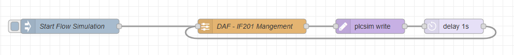
The first flowmeter loop worked because each node had a narrow, clear job:

1. The batch-read node refreshed the cached source values.
2. The first function node selected the source that should drive the instrument on that pass.
3. The second function node scaled that source into the target flowmeter value.
4. The write node pushed that calculated value back into the PLC.
5. The delay node set the pace before the next pass began.

Adding Buffered Write Mode

The next piece was changing the plcsim write node so it could work with the buffered pattern instead of always writing straight to the PLC. At first the node only had the direct path. That was fine for early proof work, but it did not fit the new batch architecture where several simulation loops might all produce outputs during the same scan.

I asked Codex to update the contrib so the write node could be switched between two modes. One mode would write immediately. The other mode would write to a buffer. When the node was set to buffer mode, it would place the output into the global context area that the buffered write loop was watching instead of sending it straight out through the bridge.

That gave the flow a much cleaner handoff. The simulation loop could finish its calculation and publish the intended output into the buffer. The dedicated buffer-write node could then take responsibility for sending that value to the PLC on the proper write pass.

The other useful detail was what happened afterwards. Once the buffer-write node had pushed that value into the PLC, it would remove the stored context entry so it could not be written again by accident on the next pass. That kept the buffer acting like a queue of pending changes rather than a list of stale writes waiting around forever.

With that in place, the whole flow had settled into a much more robust shape. The read side refreshed the cached PLC state every scan. The simulation logic worked from that cached state and updated the output buffer. The buffered write path then pushed those pending changes back into the PLC and cleared them once they had been sent.

1. The batch-read side refreshed the live values on each scan.
2. The simulation loop calculated the next output from those cached values.
3. The write node placed that output into the buffer context when buffer mode was selected.
4. The buffer-write node sent the pending output to the PLC.
5. The buffer entry was removed after the write so it would not be sent again.

Moving To Asset-Specific Simulation Nodes

The next refinement was making the simulation functions asset specific. That was the same line of thinking behind Asset Oriented Programming. A flowmeter does not need the same behaviour as a level. A pressure signal has its own rules again. Once the read, calculate, and write pattern was working, the next sensible step was to package that behaviour around the asset type itself.

Course

Asset Oriented Programming In Siemens TIA Portal

If you want to see this type of asset related management in a real project then this course takes you through large scale adoption of this method in actual PLC control environments.

Explore The Course

I used Codex again here, this time to help build a dedicated flowmeter contrib node. The goal was to stop wiring the whole behaviour together out of separate functions every time and instead let the flowmeter logic live inside a node that already understood what a flowmeter needed.

That node could accept the JSON config on the node itself. The same ideas were still there, they had just moved into a more natural home. The node could hold the source list, the output definition, the write mode, and the operating options without me having to rebuild that structure around it in the flow on every use.

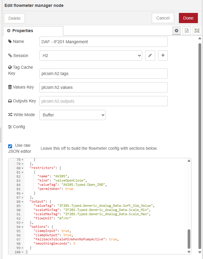
The useful part of that step was how specific the node could become. A flowmeter asset needs sources that can drive it, such as pumps. It also needs restrictions that can change the available flow, such as valves. Those restrictions could then shape how the flowmeter responded to the wider process around it instead of only following a raw speed signal.

If you look at the flowmeter contrib node itself, you can see that shape clearly. It has a place for the shared session, the cached values, the outputs buffer, the write mode, and the asset config. Inside that config, the node can hold sources, restrictors, output tags, and the options that control the simulation behaviour.

That was a useful change in direction for the project. The flow still carried the process logic, but the asset-specific rules no longer had to live in loose function nodes. The flowmeter node could accept its own config and act like a proper simulation building block inside the contrib package.

Refining The Flowmeter Response

Once the flowmeter node had settled into place, I could start tuning how it behaved across the operating range. The first version used a direct relationship between source value and output. Later on, I added flow curves to the node config so each source could describe several points across that range and let the node work between them.

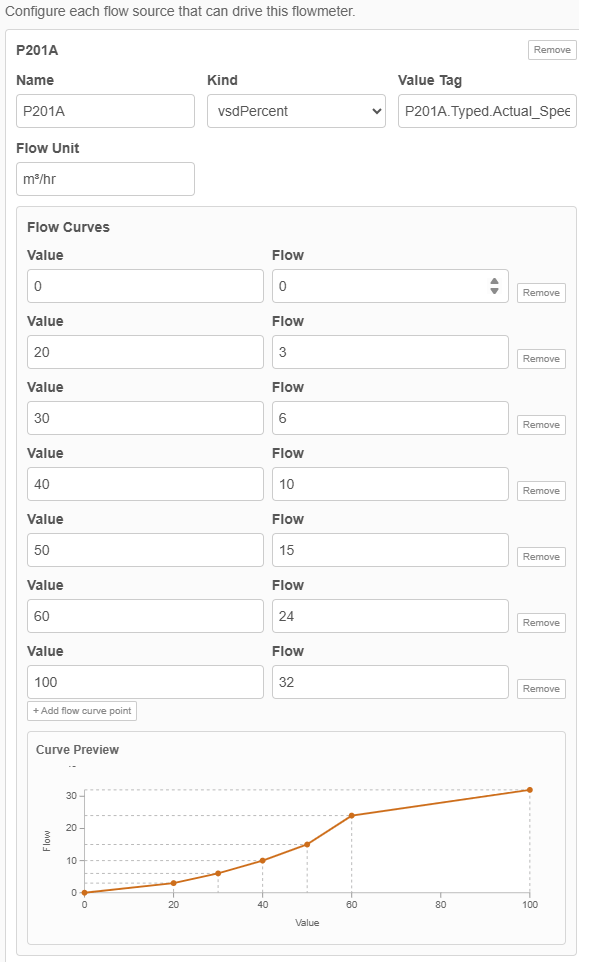
That suited the flowmeter problem much better. Pump behaviour is rarely a straight line from zero to full output, and different assets often need different shapes. Putting those points into the node config meant I could tune IF201 inside the node itself while keeping the surrounding pattern exactly the same. The batch-read side still refreshed the live values, the manager still worked from the shared buffer, and the buffered write path still sent the result back to the PLC.

Adding A Level Controller

By this point the flow simulation had started doing proper work. I could see IF201 changing as P201A or P201B ramped up and down, and that only happened when AV205 was open because the flow took a different route otherwise. The pumps were being controlled by the PLC, the simulated flow was feeding back into that control, and the PID could now drive the pumps toward a target flow setpoint through a closed loop that ran across the PLC and the Node-RED simulation together.

The next layer was level. Those pumps were not just making a flowmeter move. They were drawing from one tank and pushing into another, and my pump start and stop logic depended on those levels. I wanted the levels to rise and fall with the process in a way that was relative to the flow already being simulated. Using the flowmeter value would be ideal, but pump speed was good enough as a first practical relationship because the goal here was to test behaviour rather than chase perfect hydraulic accuracy.

I asked Codex to create a level controller in the same style as the flowmeter node. The level problem needed a looser model than the flowmeter though. A tank might fill from a pump, a valve, another part of the process, or just a fixed background rate. It might empty through one device or several. So the node had to accept separate sources and draws, along with the usual session, cached values, outputs key, and write mode.

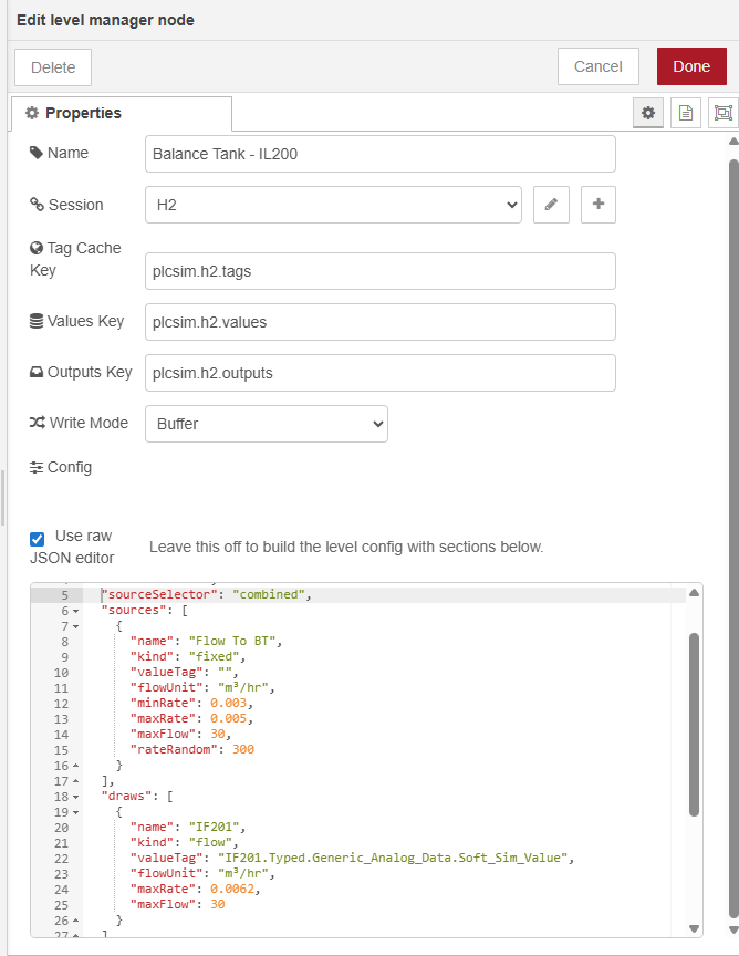
Version one went straight into Node-RED. I updated the tag config, wired in the new level node, and set the tank drawdown so that when P201A or P201B were pumping there was a linear relationship between pump activity and the rate at which the tank dropped. The source of that tank was out of scope for the project I was working on, so I added a random fill input as a stand-in. Every few minutes that random input would shift, which meant the tank had a changing refill rate rather than sitting on a fixed artificial number.

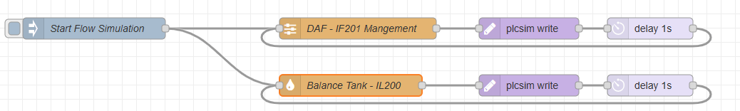
That gave me a much better test bed for the pump control. The pumps could start under PLC control, draw the tank down while they were running, and stop again when the level conditions were met. When they were off, the random fill source could bring the tank back up. At that point I was no longer just proving one instrument at a time. I had enough process behaviour in place to test how the pumps responded to the wider plant conditions around them.

1. The batch-read side refreshed the latest pump, valve, flow, and level tags.
2. The flowmeter loop updated IF201 from the pump relationship and the valve condition.
3. The level node calculated how quickly the tank should fall or recover on that pass.
4. The buffered write path sent the new simulation values back to the PLC.
5. The PLC could then act on those changing values in the next control pass.

Hardening The Simulation And Repeating The Pattern

By then I had a working pattern for the flowmeter and a working pattern for the level, and the next step was to apply that same approach to other asset types. Each asset still needed its own rules, but the wider structure was now in place. The live state came into the buffer. The asset logic ran from buffered values. The intended outputs were published, and the managed write path sent them back to the PLC.

By then I could watch IF201 change as the pumps ramped, see the tank level rise and fall around that activity, and see the PLC react to those values in return. At that point the simulation was already useful for testing. The next focus was keeping it dependable enough to extend across more of the plant.

One of the first hardening jobs was the loop guard. If the PLC connection failed and then came back, I did not want an old loop and a restarted loop both circulating at the same time. That would leave duplicate messages chasing each other around the internal simulation path and the behaviour would drift very quickly. So I added a guard so that when communications dropped and were re-established, the simulation loops could start cleanly instead of spawning a second pass on top of the first.

I also added a monitor around the communications path so the flow could detect when that link had failed and bring it back up again without me having to manually rebuild the whole chain. That sat alongside some cleaner grouping and colouring in the Node-RED workspace, which helped a lot once the flow had grown large enough that I needed to read it, troubleshoot it, and keep extending it over time.

By then, adding a new piece of simulation behaviour followed a steady rhythm.

1. Decide what the asset needed to respond to and what it needed to drive.
2. Add the required tags to the batch-read config so the live state was always available.
3. Build the asset logic around buffered values and buffered outputs.
4. Protect the loop so comms failures and reconnects did not leave duplicate passes running.
5. Drop the new asset into the wider flow and let the shared read and write paths handle the traffic.

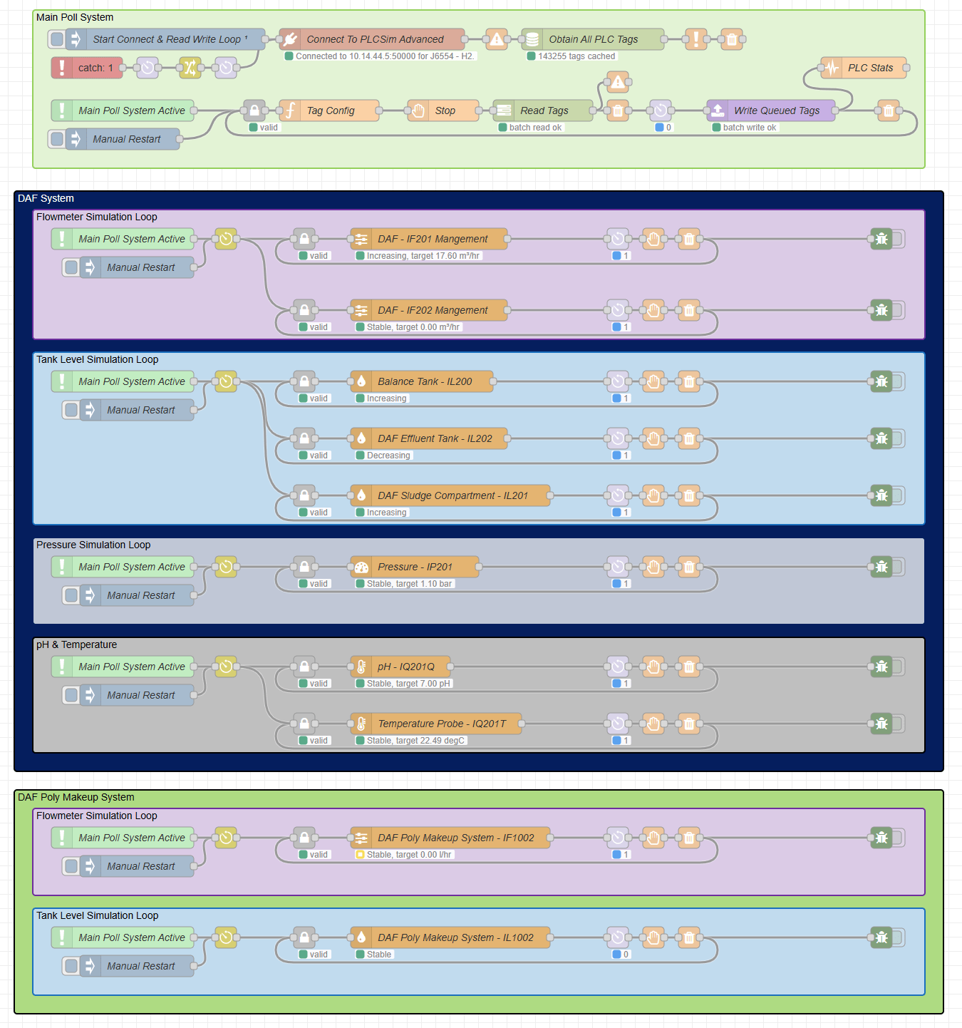
That same pattern carried on into the rest of the simulation. Flow led into level. Level led into pressure. Pressure led into slower analog signals such as pH and temperature. The wider flow also picked up extra plant areas, extra loops, and more grouped sections, but the structure underneath stayed familiar. One shared buffer for reads. Asset loops working from that buffer. Outputs queued in one place. One managed write path sending them back to the PLC.

That is where the article really lands. It started with a simple question about whether Node-RED could talk to PLCSIM Advanced at all. It ended with a reusable simulation architecture that could hold a live PLC session open, read and validate tags, model asset behaviour, recover from communications drops, and keep expanding as the project asked for more. Each layer solved the next constraint before the next one was added, which is why the later simulation sections had something dependable underneath them.

Where To Take It Next

If you want to build something similar, start with the smallest closed loop you can prove properly. One connection. One read path. One write path. One asset relationship that you can watch working from end to end. Once that holds together, the rest gets much easier to grow because every new asset can plug into a structure that already knows how to read, write, restart, and recover.

A simulation can become useful long before it covers a whole plant. One flowmeter and one tank can already tell you a lot about pump sequencing, level control, interlocks, and operator behaviour. Some jobs only need a handful of soft-sim values so a sequence can be proven before site work. Other jobs benefit from a much wider sandbox where pumps, tanks, pressure signals, chemical dosing, alarms, and operator actions can all be exercised together.

That open-ended part is what makes this approach worth exploring. You can keep the model rough and practical, or keep refining it until the relationships look much closer to the real process. You can keep it focused on one skid, one system, or one unit operation, or build outward until you have a much broader test environment. The structure now supports both directions, so the next step is mostly down to what you want to prove.

So that is probably the best place to leave this one. If you are curious about doing the same thing, start small, get one relationship working properly, and keep layering from there. Node-RED and PLCSIM Advanced are enough to build a genuinely useful simulation environment once the read path, write path, buffering, and asset structure are in place. From there it can grow as far as the project, the budget, and your curiosity make it worth taking.