A practical beginner’s guide to PLC I/O, from pushbuttons and proximity sensors through to 4-20mA transmitters, output types, wiring basics, addressing, troubleshooting, and the habits that make field signals easier to understand.
When people first get into PLCs, they often spend a lot of time learning software and not quite enough time learning how the software connects to the real machine. You can become familiar with contacts, coils, timers, and function blocks, but still feel unsure when somebody points at a terminal strip and asks, “Which input is that sensor on?” or “Why is this output on in the code but the valve is not moving?”
That gap is where a lot of early confusion lives. PLC programming feels abstract until you understand inputs and outputs properly. Once I/O starts to click, the controller stops feeling like a mysterious box full of addresses and starts to feel like a very logical interface between electrical signals and machine behaviour.
If scan cycles explain the rhythm of a PLC, inputs and outputs explain its senses and its hands. Inputs tell the PLC what is happening. Outputs let the PLC influence what happens next. Everything else in the program sits between those two points.
So this article is going to stay grounded. We will look at what inputs and outputs really are, the difference between digital and analog signals, common device types, how addresses and tags fit in, what source and sink wiring actually mean, why output hardware type matters, how to trace a signal on a drawing, and how to troubleshoot the sort of faults you will meet in real panels and real machines.
Inputs And Outputs
At the most practical level, an input is a signal coming into the PLC from the outside world, and an output is a signal going out of the PLC toward the outside world.
That sounds obvious, but there is a more useful way to frame it. Inputs are how the PLC learns about conditions. Outputs are how the PLC issues commands. Every PLC program, no matter how large or small, is constantly doing some version of the same job:
- Read the state of field inputs.
- Decide what should happen.
- Write commands to field outputs.
The word field matters here. In automation, “field” normally means the real hardware out on the machine or plant, not the PLC memory. That includes pushbuttons, selector switches, limit switches, photoelectric sensors, proximity sensors, pressure switches, transmitters, valve positioners, contactors, solenoids, beacons, and countless other devices.
One of the most important early distinctions is between the device and the signal. A PLC input is not directly reading “a level is high” or “the door is closed.” It is reading an electrical condition at a terminal. Maybe that condition was created by a float switch closing, maybe by a prox sensor switching 24VDC, maybe by a pressure switch opening a contact, maybe by a 4-20mA transmitter increasing current. The PLC only knows the electrical result presented to its input circuitry.
The same applies on the output side. A PLC output is not physically “starting a motor” in the abstract. It is switching an electrical output. That output might energise a relay coil, which energises a contactor coil, which closes power contacts, which allows a motor to run. Or it might send a 4-20mA speed reference to a drive. Or it might switch a solenoid valve. The PLC issues a signal. The field hardware and power circuit turn that signal into action.
That distinction becomes extremely useful once you start troubleshooting. If a motor is not running, the question is rarely “Is the PLC bad?” The better question is “Where in the signal chain is the expected condition being lost?” If a tank level is wrong on the HMI, the question is “What is the actual field device sending, what is the input module receiving, and what is the program doing with that value?”
It helps to picture I/O as a chain rather than a single point. For an input, the chain usually looks something like this:
- A field device changes state or measured value.
- That change appears electrically on the wiring.
- The PLC input module detects it.
- The PLC copies it into memory.
- Your logic uses that stored value.
For an output, the chain is the reverse:
- Your logic decides an output command should be on, off, or set to a value.
- The PLC writes that result to the output module.
- The output module switches voltage, current, or a contact.
- The field device responds.
- The machine changes state.
Once you start thinking in chains, a lot of uncertainty clears up. You stop treating an address in the code as if it is the whole truth. You start asking whether the field device is correct, whether the wiring is intact, whether the module LED agrees, whether the software address is right, whether the logic is using the signal correctly, and whether there is any feedback proving the command actually caused the physical result.
Note: the PLC does not directly understand pumps, valves, or tanks. It understands electrical signals that represent conditions and commands. That is why clear I/O design and good naming matter so much.
Digital Inputs
Digital inputs are the easiest place to start because they only have two meaningful states. On or off. True or false. 1 or 0. Open or closed. The wording changes from one platform to another, but the basic idea stays the same.
If you press a start pushbutton, a digital input changes state. If a guard switch closes, a digital input changes state. If a prox sensor sees metal, a digital input changes state. If an overload auxiliary contact opens, a digital input changes state. In each case the PLC is not measuring a smoothly varying quantity. It is detecting whether an electrical threshold has been crossed in a way the module interprets as on or off.
That is why digital inputs are sometimes called discrete inputs. They represent distinct states, not continuous values.
Common digital input devices include:
- Pushbuttons and selector switches.
- Limit switches and door switches.
- Proximity sensors and photoelectric sensors.
- Float switches and pressure switches.
- Auxiliary contacts from contactors, overloads, and relays.
- Status contacts from drives, soft starters, and packaged equipment.
What they all have in common is that the PLC sees a changed input state, even though the field devices themselves may work in different ways. A pushbutton is a mechanical contact. A prox sensor is electronic. A pressure switch uses a process condition to operate an internal contact. A drive healthy contact might be generated inside another control device altogether. The input module does not care about the backstory. It only responds to the electrical signal it receives.
That last point is worth pausing on because it clears up a lot of beginner questions. A PLC digital input does not know why it is on. It only knows that the voltage or current at that channel is in the range that means “on” for that module. Interpreting what that means in the machine context is the job of the program, the naming, the documentation, and the human reading it.
Most modern control panels use 24VDC digital inputs, especially for sensors and control devices. That is common because it is relatively safe, practical, and easy to distribute through control hardware. You will still see other voltages in industry, including 120VAC inputs on some systems, but 24VDC is the everyday baseline for a huge amount of modern PLC work.
| Field device | What is happening physically | What the PLC sees | Typical use |
|---|---|---|---|
| Pushbutton | An operator presses or releases a contact | Input turns on or off | Start, stop, reset, jog |
| Proximity sensor | Sensor detects metal target | Input turns on or off | Position detection, counting, presence check |
| Limit switch | Mechanical arm or plunger changes contact state | Input turns on or off | End-of-travel proof, gate position |
| Pressure switch | Pressure crosses a setpoint and changes a contact | Input turns on or off | Low pressure alarm, pump permissive |
| Contactor auxiliary | Contactor changes auxiliary contact with coil state | Input turns on or off | Run feedback, interlock, status |
There are a few practical distinctions inside the digital-input world that are worth understanding early.
Maintained versus momentary is one. A maintained device stays in its new state until something changes it again. A selector switch in Hand or Auto is a good example. A momentary pushbutton only changes state while you are pressing it. In the code, those two behaviours often need different treatment. A momentary start pushbutton may need edge detection or a seal-in circuit. A maintained permissive usually just needs to be true whenever the system is allowed to run.
Normally open versus normally closed is another. This is about the device’s contact state in its normal, unoperated condition. It is not the same thing as whether the machine is safe or unsafe. A normally closed stop pushbutton is common because opening that circuit indicates a stop condition. A normally open start pushbutton is common because closing the circuit indicates a request to start. The important part is to follow the actual drawing and device datasheet, not assumptions.
Dry contact versus wet contact also causes confusion early on. A dry contact does not supply its own voltage. It simply opens or closes a path, like a switch or relay contact. The panel wiring supplies the voltage. A wet contact or active electronic output does supply voltage from the device side. A prox sensor with a powered PNP output is a common example. Both can land on PLC digital inputs, but the wiring method is different.
Input response is another detail beginners often discover during troubleshooting rather than during training. Digital inputs are fast, but not infinitely fast. Mechanical contacts can bounce. Sensor outputs can flicker. PLC modules can have configurable filters. Fast tasks and high-speed inputs may exist for applications like counting encoder pulses or seeing very short events. If a signal is only present briefly, whether the PLC sees it can depend on scan time, hardware filter time, and the input type being used.
Good habit: when you are checking a digital input fault, compare four things together: the physical device state, the module LED, the online software state, and the way the tag is used in logic. If one of those does not agree with the others, you have already narrowed the problem down.
Digital Outputs
Digital outputs are the other half of the basic I/O picture. Where digital inputs tell the PLC about on/off conditions, digital outputs let the PLC send on/off commands.
If a stack light turns on, a buzzer sounds, a solenoid valve energises, a contactor coil pulls in, a pump start relay closes, or a conveyor enable signal is sent to another panel, you are usually dealing with some form of digital output.
Just as with inputs, the first useful distinction is between the command and the final physical action. The PLC output might only be energising a small interface relay. That relay might then switch a larger current to a contactor coil. The contactor then closes power contacts to feed a motor. So when the output bit is true in the PLC, what you have immediately proven is that the controller is trying to command that path. You have not yet proven that the downstream hardware successfully responded.
This is why experienced programmers like feedback signals. If you command a motor contactor on, it is useful to have an auxiliary contact back to the PLC proving the contactor actually pulled in. If you command a valve open, it is useful to have an open limit switch confirming movement. Output commands are necessary. Feedback makes them trustworthy.
Common things driven from digital outputs include:
- Indicator lights, beacons, sirens, and buzzers.
- Interposing relays and contactor coils.
- Solenoid valves and pneumatic pilots.
- Enable signals to drives, burners, and packaged equipment.
- Panel interface signals to other PLCs or remote systems.
Output hardware type matters here. The two common categories are relay outputs and transistor outputs.
Relay outputs use a mechanical contact inside the output module. They are flexible because they can usually switch AC or DC within their ratings, and they isolate the PLC electronics well. They are slower than solid-state outputs and have a mechanical life limit because contacts physically move and wear. For many general-purpose control duties they are still perfectly appropriate.
Transistor outputs are solid-state DC outputs. They are common on modern PLCs, especially where fast switching is useful. They switch quickly, do not have contact wear in the same way as relays, and are a good fit for many 24VDC control tasks. They do, however, have polarity considerations, and they are not interchangeable with AC output needs.
| Output type | Best suited to | Strengths | Watch-outs |
|---|---|---|---|
| Relay | General-purpose AC or DC switching | Flexible, isolated, easy to understand | Slower, contact wear, limited life under heavy switching |
| Transistor | 24VDC and fast switching applications | Fast, no mechanical contact wear, common on modern panels | DC only, polarity matters, output ratings still apply |
Ratings matter just as much as type. Every output has limits for voltage, current, and often surge or inrush behaviour. That last part catches people out. A coil or lamp may have a modest steady-state current but a higher startup current. A solenoid may generate inductive kick when de-energised. A relay output may handle a pilot relay comfortably but not a larger field load you hoped would be “close enough.”
That is why you will see interposing relays used so often. They let the PLC output switch a smaller, well-understood control load, and let a separate device handle the field-side switching duty. They are not always necessary, but they are common for good reason.
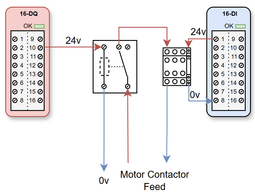
This kind of visual helps show why an output bit being true is not the same as a motor being physically confirmed as running.
There is also a subtle but important software side to digital outputs. In logic, an output tag often represents the commanded state. In a well-structured program, the actual device status may come back on separate feedback inputs. Mixing those two concepts together causes trouble. A commanded-on pump and a proven-running pump are related, but they are not the same signal and they should not be treated as if they are.
// Example of separating command from feedback
P100_Start_Command := AutoRequest AND PermissivesOK AND NOT FaultActive;
Q_MotorContactor := P100_Start_Command;

// Separate input proving the field device responded
P100_Running_Feedback := I_MotorAux;

// Alarm if commanded on but not proven within time
IF P100_Start_Command AND NOT P100_Running_Feedback THEN
    StartFeedbackFaultTimer(IN := TRUE, PT := T#3s);
END_IF;
That pattern appears everywhere in industrial control because it reflects reality well. The PLC can command. The field must confirm. If you make that separation clear in your code and your I/O naming, troubleshooting gets much easier for the next person.
Analog Inputs And Outputs
Digital I/O gives you two states. Analog I/O gives you a range.
An analog input lets the PLC measure a continuously changing quantity such as pressure, level, temperature, flow, speed, weight, or position. An analog output lets the PLC send a continuously variable command such as valve position demand, drive speed reference, or proportional control signal.
This is where a lot of newcomers feel a jump in difficulty, but the principle is still straightforward. Instead of asking, “Is the signal on or off?” the PLC is now asking, “What value is this signal currently representing?”
A pressure transmitter might send 4mA at 0 bar and 20mA at 10 bar. A level transmitter might send 4mA at an empty tank and 20mA at a full tank. A drive speed reference output might use 0-10V where 0V means stopped and 10V means full speed. The PLC module measures that electrical signal and converts it into a number in memory.
That number is often not yet in human-friendly engineering units. Many PLCs first store an internal raw value that depends on module resolution and configuration. Your program may then scale that raw value into bar, litres, percent, degrees Celsius, or some other useful unit. Different platforms hide more or less of this process, but the concept is universal.
In practical terms, analog I/O usually involves four layers:
- The process variable in the real world, such as 6.2 bar or 48 percent level.
- The transmitter or output device converting that into voltage, current, resistance, or another signal form.
- The I/O module converting that signal into a digital number the PLC can work with.
- The program scaling and interpreting the number.
So if a tank level reading looks wrong, there are several places the problem might be. The tank may really be at a different level than assumed. The transmitter may be misranged. The wiring may be wrong. The module may be configured for the wrong signal type. The scaling in the code may be off. The HMI may be displaying the wrong tag. Analog troubleshooting is not harder because analog is mysterious. It is harder because there are more stages where a mismatch can happen.
The two analog signal forms beginners meet most often are 0-10V and 4-20mA.
0-10V is easy to visualise. Zero volts represents the low end of the range, ten volts represents the high end, and values in between represent points between the two. It is common in some devices and some control schemes, especially on shorter runs or within cabinets.
4-20mA is extremely common in industry because current loops handle longer distances and electrical noise well. The reason 4-20mA became such a standard is very practical. A current loop is less sensitive to voltage drop over long cables than a voltage signal. Also, because the “live zero” starts at 4mA rather than 0mA, you can distinguish a genuine low reading from a dead circuit more easily. If you are expecting 4-20mA and you measure 0mA, that often points to a fault such as a broken wire or lost power rather than a legitimate process value.
That live-zero concept is worth understanding early. In a 4-20mA level transmitter scaled 0 to 100 percent, 4mA represents 0 percent and 20mA represents 100 percent. If the wire breaks and the current drops away completely, the PLC does not confuse that with 0 percent level unless the design or scaling is poor. That is one reason 4-20mA remains so popular.
Why 4-20mA is everywhere: it is robust over distance, reasonably noise resistant, and the 4mA live zero makes fault detection easier than a signal that starts at 0mA.
Not all analog inputs are voltage or current. Temperature is a good example. An RTD changes resistance with temperature. A thermocouple generates a small voltage related to temperature. Load cells and some specialist instruments use other measurement principles again. The idea is still the same. A real physical quantity is being translated into a signal the PLC module can measure.
On the output side, analog signals let the PLC command something more nuanced than on or off. A control valve may need to open 35 percent, not simply open or closed. A VFD may need a speed demand of 43Hz or 72 percent of reference. A proportional hydraulic valve may need a smoothly varying command. That is where analog outputs become useful.
// Example of simple 4-20mA scaling to percent
// 4mA = 0%, 20mA = 100%
LevelPct := ((Level_mA - 4.0) / 16.0) * 100.0;

// Clamp to protect downstream logic from bad values
IF LevelPct < 0.0 THEN LevelPct := 0.0; END_IF;
IF LevelPct > 100.0 THEN LevelPct := 100.0; END_IF;
That code example is deliberately plain, because the point is the concept. The PLC receives a signal, turns it into a number, scales it into engineering units, and then logic can use that value meaningfully.
There are some practical analog habits that make life easier:
- Always know the transmitter range, not just the process variable name.
- Check whether the module is configured for voltage, current, RTD, thermocouple, or something else.
- Make sure the engineering scale in the code matches the instrument range in the field.
- Use fault handling for out-of-range or broken-loop conditions where appropriate.
- Be cautious with filtering, because it smooths noise but also delays response.
In my experience, analog problems are rarely solved by staring only at the HMI value. You need to know what the field instrument should be sending, what the PLC channel is configured to receive, and how the raw or scaled value is being interpreted. Once you break the problem into those layers, analog I/O becomes much more manageable.
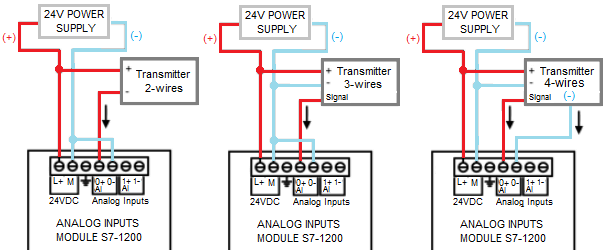
Image credit: electricalchilean.cl.
Addressing And Tags
Once you understand what I/O devices do electrically, the next question is how the PLC refers to them in software.
Every physical I/O point needs some kind of unique identity. On older or more direct systems, that identity may be a hardware address such as I0.0, %I0.3, Q4.2, or something similar. On more tag-based platforms, you may be looking at names like Local:1:I.Data.0 or descriptive tags that hide the raw address almost completely.
The details vary by platform, but the underlying concept is simple. The software needs a reliable way to connect a signal in memory to a real point on real hardware.
For beginners, one of the first useful things to understand is that the raw hardware address and the descriptive tag are not enemies. In good projects, they work together. The raw address connects you to the hardware. The descriptive tag connects you to the machine meaning.
For example, an address like I0.4 tells you that the point is on an input byte and bit position somewhere in the hardware map. A tag like P100_Running_Feedback tells you what that signal means to the process. If you only use raw addresses, the code becomes hard to read. If you only use descriptive names without any disciplined mapping to hardware, fault-finding and commissioning can become messy. The best projects usually create a clear bridge between the two.
| Platform style | Example | What it tells you |
|---|---|---|
| Direct bit address | I0.0 | Input area, byte 0, bit 0 |
| Percent-style address | %Q4.2 | Output area, byte 4, bit 2 |
| Chassis/module style | Local:2:I.Data.5 | Specific module slot and input bit |
| Alias or symbolic tag | IL100_High_Level | Human-readable machine meaning |
This is also where the scan cycle comes back into the picture. Most PLCs read physical inputs, copy them into an internal memory image, run the logic using that image, and then update physical outputs from the output image. That means when you look at an input tag in the program, you are normally looking at the PLC’s current stored representation of that input, not a direct electrical meter probe into the terminal every line of code.
That matters because it explains why execution order, filters, and task timing matter. It also explains why an output being true in logic does not always guarantee the field device has moved yet. The program command is one stage. The hardware response is another. If you need proof, use feedback.
A lot of projects benefit from an I/O mapping layer. That means the raw addresses are read in one part of the program and assigned to descriptive tags that the rest of the code uses. Likewise, internal command tags may be mapped to physical outputs in one place. The idea is to keep hardware representation and process logic separate enough that the code stays readable and changes stay manageable.
// Example of a simple mapping approach
Start_Pushbutton := I0_0;
Stop_Pushbutton := I0_1;
P100_Running_Feedback := I0_2;
IL100_High_Level := I0_3;

P100_Start_Command := AutoDemand AND SystemHealthy;

Q0_0 := P100_Start_Command;
Q0_1 := Alarm_Beacon_Command;
On larger systems, the mapping can become more structured than that, especially when remote I/O, device diagnostics, or object-oriented equipment modules are involved. But the beginner-friendly idea is the same. Give meaningful names to signals. Keep a trustworthy link to hardware. Avoid scattering raw addresses everywhere if it makes the program harder to follow.
Remote I/O does not change the concept, only the transport. A sensor may physically land on a remote rack over PROFINET, EtherNet/IP, EtherCAT, or another network rather than on the CPU’s local terminals. To the logic, it is still an input value arriving from hardware. The important part is still correct addressing, clear naming, and reliable diagnostics.
I/O Wiring Fundamentals
Wiring is where many I/O misunderstandings become very real. You can have perfect logic and still have a dead signal if the panel wiring, device type, common reference, or polarity is wrong.
The first thing to keep straight is that words like common, 0V, neutral, and earth are not interchangeable just because they all sound like “the return side.”
In a typical 24VDC control panel, 0V is the DC return reference. A module common terminal may connect to 0V or 24V depending on whether the input scheme is sinking or sourcing. Neutral is an AC supply conductor. Earth is protective grounding. Mixing those ideas mentally leads to wiring mistakes and bad troubleshooting assumptions.
Then there is the famous sourcing and sinking question, often discussed alongside PNP and NPN. This topic gets overcomplicated in a lot of explanations, so here is the practical version.
A sourcing device provides the positive voltage to the load or input. A sinking device provides a path back to 0V. In the sensor world, PNP outputs are generally sourcing and NPN outputs are generally sinking. In many modern 24VDC PLC systems, especially on European-style equipment, PNP wiring is very common. But you should always confirm the actual device and module design, not rely on habits or geography.
What matters in the field is compatibility. A PLC input wired to expect a sourcing device will not behave properly if you connect a sinking sensor to it without the correct arrangement. This is why the input module common and the sensor output type both matter. It is not enough to know that “a prox sensor is installed.” You need to know what kind.
Dry contacts add another layer. A dry contact device such as a relay auxiliary or limit switch does not source voltage itself. You must provide the switching voltage through the wiring. In a 24VDC input circuit that often means routing 24V through the device and back to the input, or using the opposite arrangement depending on module type. The contact is just opening or closing a path.
Electronic sensors usually need power as well as a signal connection. A three-wire DC prox sensor often has +24V, 0V, and switched output. A two-wire transmitter may draw its operating power from the current loop. A four-wire device may separate power and signal. These are not details to skip. They determine whether the input module ever sees a valid signal at all.
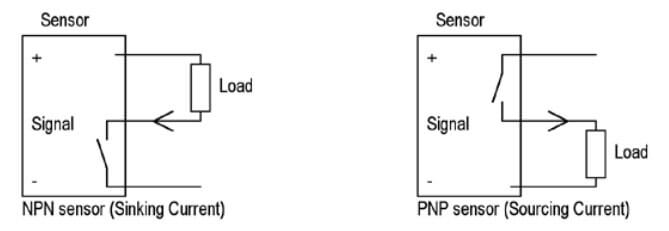
Image credit: Automation Ready Panels. Read their article NPN vs PNP.
Polarity matters on many signals. Reverse the polarity on a DC sensor and it may not power up. Reverse a current loop connection and the PLC sees nothing or sees a fault. Wire a transistor output the wrong way around and the load may never switch. Beginners sometimes treat control wiring as if every signal were just “a wire from A to B.” On real systems, the direction of the electrical reference matters.
Output wiring has its own version of the same lesson. A PLC output might switch the positive side of a DC load, or the return side, depending on module design. A relay output may simply present a contact and require you to bring your own supply through it. A transistor output may need the right common terminal arrangement to switch properly. Reading the module wiring diagram is not an optional extra. It is part of the job.
For analog loops, it also matters whether the instrument is 2-wire, 3-wire, or 4-wire. A 2-wire 4-20mA transmitter is powered by the loop and signal path together. A 4-wire device may have separate power and analog output terminals. If you wire one as if it were the other, the signal will not behave.
In practice, the best beginner habit is this: before assuming the code is wrong, make sure you can sketch the actual field circuit in plain language. Where is the supply? Where is the return? What changes state? What terminal should go high, low, open, closed, or carry current when the device operates? That small discipline catches a huge number of faults early.
Another practical habit: if a signal “makes no sense,” stop describing it in software terms for a moment and describe it electrically instead. Ask what voltage or current should be present, where it should be present, and what reference it is measured against.
Reading Drawings And Following A Signal From Device To Code
One of the biggest jumps in confidence comes when you can move comfortably between electrical drawings, panel hardware, and PLC software without feeling like they are three separate worlds. That is really what I/O understanding is for.
Suppose you have a tank high-level switch. On the drawing, it may have a device tag. That device tag lands on a terminal strip. From there a wire goes to an input card channel. The I/O schedule tells you that channel corresponds to a PLC address. In the PLC program, that address is mapped to a descriptive tag. The logic uses that tag to stop a filling valve and generate an alarm. On the HMI, that alarm is shown to the operator.
If you can follow that chain in both directions, you are in a strong position. If the alarm is active unexpectedly, you can trace backward from the HMI to the logic, to the tag, to the address, to the module terminal, to the field device. If the tank really is high and the valve did not close, you can trace forward from the switch state through the PLC input, through the logic, through the output command, and out to the valve solenoid.
I/O schedules are especially helpful here. A decent I/O schedule will tell you the point description, address, module location, signal type, and often the field device tag. It becomes the bridge between design documentation and live troubleshooting. When documentation is poor, this is often the missing piece that makes simple faults take much longer than they should.
There is a very practical sequence you can use when following a digital signal:
- Identify the field device and what state it should be in physically.
- Check the wire or terminal path on the drawing.
- Check the I/O module channel and LED.
- Check the PLC address or mapped tag online.
- Check how the logic uses that signal.
- Check the output command and any related feedback.
Experienced engineers do this almost automatically. They are not guessing. They are narrowing the problem by walking the signal path. The good news is that this is a skill you can practise deliberately. Every time you look at a real I/O point, ask yourself where it lives on the drawing, what address or tag it uses, and what the PLC must be seeing for the logic to behave the way it does.
Once you build that habit, even unfamiliar systems become much less intimidating. They may use different hardware or different naming conventions, but the signal still has to travel from a device, through wiring and I/O, into logic, and back out again.
Troubleshooting I/O Problems
Most real I/O faults are not glamorous. They are loose wires, wrong addresses, blown fuses, incorrect scaling, dead sensors, bad commons, mismatched device types, or output paths that are only half-understood. The reason these faults can still consume a lot of time is that people jump around instead of tracing the signal methodically.
Digital input faults are a good example. Let us say a limit switch “does not work.” That could mean the switch itself is damaged. It could mean the actuator no longer hits it. It could mean the switch is fine but the wire is loose. It could mean the input card channel is wrong. It could mean the PLC sees the signal correctly but the logic uses the wrong tag. It could mean the signal is correct and the real problem is that another interlock still blocks the sequence. The phrase “does not work” is too vague to be useful until you narrow where the chain breaks.
A good digital input checklist looks like this:
- Is the field device physically changing state?
- Is the correct voltage or continuity change present at the terminal?
- Does the module LED change?
- Does the PLC input tag change online?
- Does the logic react the way the design says it should?
If the module LED does not change, you are likely dealing with field wiring, power, or the device itself. If the LED changes but the software tag does not, the addressing or configuration may be wrong. If the software tag changes but the machine does not react, the problem is probably in logic, sequence conditions, output path, or downstream hardware. That kind of structured thinking is much faster than bouncing between random theories.
Output faults follow the same logic in reverse. Suppose a pump will not start. Check whether the PLC output command is actually being issued. Check whether the output channel LED is on. Check whether the correct voltage appears at the output terminal. Check whether an interposing relay or contactor coil is receiving that signal. Check whether overloads, safeties, or local isolators are preventing action. Check whether there is run feedback. Starting at the output and working outward is often the quickest route.
In my experience, a surprising number of “PLC output faults” turn out to be field power issues, coil failures, blown protection devices, or external interlocks. The PLC bit being on only proves the command exists in the controller. It does not prove the field side completed the job.
Analog faults benefit from the same discipline. If a level reads backwards, check whether the transmitter range or polarity is wrong. If the reading is stuck, measure the signal at the terminals and compare it to the real process. If the value is noisy, consider shielding, grounding, filtering, and sensor health. If the value is offset, check calibration, module type, and engineering scaling. “The analog is wrong” is not a diagnosis. It is a starting point.
There are also time-related I/O problems. A contact bounces. A prox pulse is too short. An input filter delays recognition. A relay output wears and becomes intermittent. A networked I/O node updates slower than expected. A transmitter is heavily damped. The signal path may be correct in principle, but the timing still produces bad behaviour. This is where understanding scan cycles and response times helps you ask sharper questions.
Fast input means different things on different platforms, but broadly it means hardware or tasks designed to capture short events more reliably than normal cyclic logic. That matters for encoders, counters, registration marks, and other fast-moving processes. For ordinary pushbuttons and limit switches, standard input handling is usually enough, but contact bounce and filter settings still matter.
Forcing I/O in software can help with troubleshooting, but it should be used carefully. Forcing an input can help you prove whether logic reacts. Forcing an output can help you prove whether a field device responds. But forcing bypasses normal conditions, which means it can create misleading results or genuine hazards if used casually. In live industrial systems, forcing should be deliberate, documented, and done under safe conditions.
The more you can train yourself to think in signal paths rather than vague symptoms, the more quickly these problems stop feeling random.
Tip: do not ask only “what is wrong?” Ask “where was the last point in the chain that I proved was correct?” Then move one step further.
Safety I/O And The Difference Between Control And Protection
No article about inputs and outputs is complete without talking about safety, because one of the worst beginner habits is treating safety signals as if they are just ordinary I/O points with more importance attached.
Safety functions need their own design approach. Emergency stops, guard interlocks, safety light curtains, safety relays, and safety PLC logic are not just standard control inputs and outputs with stronger wording around them. They are part of a separate protective function that must be designed, validated, and maintained correctly.
At a practical level, that means you should not casually bypass safety inputs to “get the machine going,” and you should not assume a normal PLC output is an adequate safety output simply because it can switch a contactor coil. Safety-rated systems exist because the consequences of failure are different, and the design has to account for that.
Operational control logic and safety logic usually interact, but they should not be confused with each other. A standard PLC may read a safety status signal for information, alarms, or sequence behaviour. But the actual safety action of removing hazardous energy or preventing motion should rely on the appropriate safety architecture, not on standard software behaving perfectly.
This matters for I/O understanding because the drawings, modules, and diagnostics may look similar at first glance. A safety input is still an input. A safety output is still an output. But the design intent, hardware category, testing requirements, and permissible modifications are different. Treating them like normal spare control points is a serious mistake.
Good beginner habits around safety I/O are simple:
- Know whether the point you are looking at is standard control I/O or safety-related I/O.
- Do not bridge, simulate, or force safety signals casually.
- Understand that safety feedback and diagnostics often use dual-channel logic and dedicated hardware.
- Escalate changes to qualified people when safety systems are involved.
Common Beginner Mistakes With I/O
There are a handful of I/O mistakes that show up so often they are worth calling out directly.
Using the commanded output as if it were proof of action. If the PLC output bit is on, that proves the logic is requesting something. It does not prove the motor ran, the valve opened, or the contactor pulled in. Use feedback where the physical result matters.
Treating every fault as a software fault first. On a live plant, field devices, wiring, terminations, fuses, and interface hardware fail far more often than many newcomers expect. It is sensible to inspect the physical chain before rewriting code.
Ignoring naming and mapping discipline. If your code uses raw addresses everywhere, eventually it becomes hard to read and easy to misuse. If your tags are vague, you lose meaning. Good names and a consistent mapping layer turn I/O from a guessing exercise into an understandable model of the machine.
Confusing common, neutral, earth, and 0V. These distinctions matter. A lot of difficult signal faults come down to misunderstood references.
Assuming all sensors and modules wire the same way. PNP and NPN exist. Dry contacts and active outputs exist. 2-wire and 4-wire transmitters exist. Relay outputs and transistor outputs exist. Datasheets and module manuals are part of real engineering work.
Forgetting that timing matters. Inputs can bounce. Filters can delay. Outputs can wear. Analog values can be damped. Short pulses can be missed. Fast and slow behaviour both have consequences.
Not documenting spare points, moved points, or temporary changes. I/O confusion compounds over time when documentation slips. A moved wire that never made it onto the drawing becomes somebody else’s mystery fault later.
The better habits are not complicated:
- Name signals clearly.
- Separate commands from feedbacks.
- Check drawings, not memory.
- Trace signals step by step.
- Respect hardware type and ratings.
- Keep documentation current.
- Be cautious around safety I/O.
Learn More
Build PLC Code That Is Easier To Wire, Read, And Troubleshoot
If you want to go beyond individual I/O points and learn the programming structure behind maintainable control systems, my PLC and HMI Development book covers the practical engineering habits that make projects easier to build and far easier to support later.
Get the BookBuilding Real Confidence With I/O
Confidence with inputs and outputs does not come from memorising terminology. It comes from repeatedly connecting four views of the same signal: the physical device, the electrical circuit, the PLC tag, and the machine behaviour.
Being able to stand in front of a panel, look at a prox sensor, find its terminal, identify its input address, watch the corresponding bit online, and explain what the logic should do next is a strong sign that the system is starting to feel clear and readable.
If you want to improve quickly, spend time doing three things deliberately:
- Watch I/O points online while operating or simulating equipment.
- Read I/O schedules and drawings until signal tracing becomes second nature.
- Whenever a fault happens, describe the signal chain before trying random fixes.
Do that consistently and I/O stops feeling like a list of addresses and starts feeling like a language you can read.
Inputs and outputs are where the PLC meets the real world. If that layer is misunderstood, the rest of the program always feels more abstract than it needs to. If that layer is clear, ladder logic, structured text, diagnostics, and troubleshooting all become much easier to reason about.
The key takeaway is simple:
- Inputs tell the PLC what the plant is doing.
- Outputs let the PLC influence what the plant does next.
- Digital signals handle yes-or-no conditions.
- Analog signals handle measured values and variable commands.
- Wiring, module type, addressing, and feedback all determine whether those signals are trustworthy.
- Following the signal path from field device to code and back again makes PLC behaviour much easier to understand.
That is why inputs and outputs are not a small beginner topic to get out of the way quickly. They are the foundation of everything the controller can sense and everything it can command. Understand them well, and the rest of PLC programming has a much firmer base.